Approximate percentiles with t-digests

The researchers at G-Research work with ever increasing volumes of data. The data is so large that loading it all into memory can be prohibitive at best and completely infeasible at worst.

A challenge often faced is efficiently computing summary statistics for the data. While loading the data into memory might not be possible, very often the data has been sharded across many files, each of which do fit in memory.

It is not difficult to work out an algorithm for computing statistics such as the minimum or mean across all of the data without having it resident in memory. Suppose instead you are interested in knowing the 95th percentile of the data. In general, knowing the 95th percentile of the data in each shard of the data is insufficient to know the 95th percentile of the data globally.

The t-digest is a probabilistic data structure that allows accurate estimation of arbitrary percentiles of the global data without needing all of the data in memory at any one time. It works by using a simple heuristic to pick a number of points that summarise the (univariate) data well and storing this information in the digest itself. One t-digest is created per file. Then, using the same heuristic, new points are chosen that summarise all of the t-digests. From these summary points, along with some metadata, an approximate cumulative distribution can be constructed allowing percentile estimation.

The following sections explain the mechanics of each component of t-digest construction in detail.

Clustering in 1D

The t-digest relies on compressing univariate data into a small number of 1D clusters while still being representative of the overall distribution (at least approximately). A cluster is simply a collection of points on a number line as shown in Figure 1.

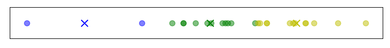
Figure 1: Example of 3 clusters in 1D.

A simple summary of a cluster is provided by its centre of mass (also called its centroid) and the number of points it contains (also called its weight). This is encapsulated in the following Python classes:

from typing import List

class Cluster:
  def __init__(self, values: List[float]):
    self._values = values

  def summarise(self) -> ClusterSummary:
    n_points = len(self._values)
    center_of_mass = sum(self._values) / n_points
    
    return ClusterSummary(center_of_mass, n_points)

class ClusterSummary:
  def __init__(self, center_of_mass: float, n_points: int):
    self._center_of_mass = center_of_mass
    self._n_points = n_points

  @property
  def centroid(self) -> float:
    return self._center_of_mass

  @property
  def weight(self) -> int:
    return self._n_points

To understand how the compression is done, it is easiest to consider the case when all of the data is available in memory. The top panel of Figure 2 shows a possible 1D clustering of 25 data points. These clusters have a property that the authors of the t-digest paper refer to as strongly ordered. A collection of clusters is called strongly ordered if a cluster with a smaller centre of mass than another is guaranteed to have all of its points be less than those of the cluster with the larger centre of mass.

This strong ordering property is visually apparent in the top facet of Figure 2. Note that all of the data points belonging to the blue cluster are less than all of the data points belonging to the green cluster. The points in the green cluster are all less than those in the yellow cluster and so on.

In contrast, the clusters in the bottom panel of Figure 2 do not exhibit strong ordering. Even though the centroid of the yellow cluster is greater than that of the green cluster, there are points belonging to the yellow cluster that are less than some of the points in the green cluster.

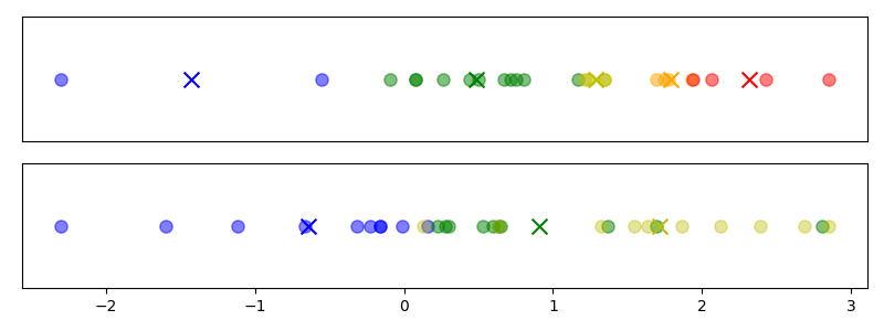
Figure 2: Top: Example of a strongly ordered cluster; Bottom: Example of a clustering that is not strongly ordered. Note that points of the same colour belong to the same cluster.

One of the main contributions of the paper is a systematic way of choosing the boundaries of the clusters. The t-digest uses what the authors call a scale function which maps a percentile to a real number, denoted by $k$. This function is used to define a criterion for how many points should be allowed in each cluster (more on this later).

When a cluster is created, the percentile of the first data point in the cluster is mapped to a $k$ value and saved. Points are continually added to the cluster (in sorted order) until enough points are added such that the $k$ value has increased by 1. At this point, the cluster is considered complete and the centroid as well as its weight are stored and a new cluster is started.

The cluster building process is shown in the animation in Figure 3. Note how there are fewer points in the clusters at the extreme quantiles where the scale function is steeper.

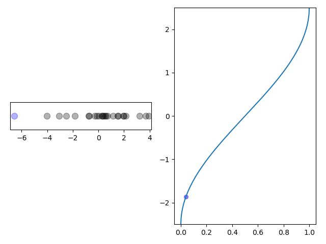
Figure 3: Left: Clusters are created by iterating through values in sorted order with a cross denoting a cluster centroid. Right: The same values mapped into $k$-space by a scale function. When the change in $k$ exceeds 1, a new cluster is started. The black crosses denote cluster boundaries.

Below is an implementation of this algorithm in Python.

import numpy as np

TAU = 2 * np.pi

def scale_fn(q: float, delta: float) -> float:
  return delta / TAU * np.arcsin(2 * q - 1)

def cluster_points(points: np.ndarray, delta: float) -> List[List[float]]:
  n_points = len(points)
  sorted_points = np.sort(points)
  data_clusters = [[]]
  k_lower = scale_fn(0, delta)
  percentile_increment = 1 / n_points
  centroids = []
  for j, pt in enumerate(sorted_points):
      percentile = (j + 1) * percentile_increment
      k_upper = scale_fn(percentile, delta)

      if k_upper - k_lower < 1:
          data_clusters[-1].append(pt)
      else:
          centroids.append(np.mean(data_clusters[-1]))
          data_clusters.append([pt])
          k_lower = k_upper

  return data_clusters

Choosing a scale function

At first glance, the choice of scale function seems complicated and arbitrary.

The first property of a valid scale function is that it must be defined over the domain $[0,1]$. This ensures every percentile is mapped to a $k$ value. However, the main property of the scale function is that it is monotone increasing. Without this property, it is possible that the change in $k$ would never exceed 1, leading to no clustering at all.

Perhaps more fundamental than the scale function itself is its derivative. The slope of the scale function determines how fast the $k$ value increases with each percentile. This effectively sets the number of points that can be added to a cluster before it is complete. The larger the slope, the fewer points will be allowed in the cluster. The smaller the slope, the more points will be included before a new cluster is started.

To make this notion more precise, consider the linearisation of the scale function $k(q)$

$Delta k approx frac{mathrm{d}k}{mathrm{d}q}Delta q$

Denoting the total number of points as $N$, the number of points in the $i$th cluster as $n_{c_i}$, and inserting the condition for finishing a cluster ($Delta k approx 1$), this becomes

$
begin{align*}
frac{mathrm{d}q}{mathrm{d}k} &approx Delta q\
&approx n_{c_i} / N\
&propto n_{c_i}
end{align*}
$

it is evident that the cluster sizes, $n_{c_i}$ are proportional to $frac{mathrm{d}q}{mathrm{d}k}$ (at least approximately).

For the arcsine scale function in the previous section, this derivative is $sqrt{q(1-q)}$. This means the extreme percentiles (near 0 or 1) will be approximated by smaller, more accurate clusters (see Figure 3).

The paper suggests four scale functions with various desirable properties

$
begin{align*}
k_0(q) &= frac{delta}{2} q\
k_1(q) &= frac{delta}{2pi} sin^{-1}(2q-1)\
k_2(q) &= frac{delta}{4 log(n/delta) + 24} logleft(frac{q}{1-q}right)\
k_3(q) &= frac{delta}{4 log(n/delta) + 21} cdot left{
begin{array}{lr}
log(2q) & q le 0.5\
-2log(2(1-q)) & q > 0.5\
end{array}
right.
end{align*}
$

Each scale function has a scale parameter $delta$ which determines the number of cluster centroids used in the compression of the CDF. Larger values of $delta$ equate to steeper scale functions. Since a steep scale function means fewer points per cluster, this translates to having many clusters. Conversely, a small $delta$ means the CDF will be approximated with fewer clusters.

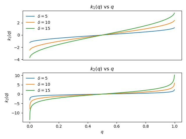
Figure 4: Different scale functions.

Defining the t-digest

The t-digest data structure is just a scale function along with a collection of cluster summaries (sorted by centroid). In order to be useful, the data structure also needs to support the following two operations:

1. Combine multiple existing t-digests into a single t-digest
2. Compute arbitrary percentile estimates

The following sections discuss each of these in more detail.

Merging digests

The preceding sections outline the case when the data fits in main memory (with some room left over to sort the data). In the scenario where each data file fits in memory, a single t-digest can be computed per file. To compute a single t-digest summarising the entire dataset, we can create a list of all the cluster summaries from each t-digest, sorted by their centroids.

The cluster summaries can then be merged in a greedy fashion by determining if the weight of the merged cluster leads to an increase in the $k$ value less than 1. If so, the two clusters can be replaced with a single merged one using the following code

def merge_cluster_summaries(c1: ClusterSummary, c2: ClusterSummary):

  w1 = c1.weight / (c1.weight + c2.weight)
  w2 = c2.weight / (c1.weight + c2.weight)

  new_centroid = w1 * c1.centroid + w2 * c2.centroid
  new_weight = c1.weight + c2.weight

  return ClusterSummary(new_centroid, new_weight)

For the most part, this algorithm is the same as the in-memory case. In the in-memory case, individual points were added to a cluster while in the merging of t-digests, clusters are added to larger clusters. Of course this is a distinction without a difference since single points can be viewed as clusters with weight 1 and centroid equal to the point’s value.

One thing that is materially different from the in-memory case is the strong ordering property. Unfortunately, when merging cluster summaries, this property is no longer guaranteed to hold. The consequence of this is error in the estimation of the percentiles.

Percentile estimation

The natural question is, “how can a t-digest be used to estimate an arbitrary percentile?”. By keeping only the centroids along with the number of points, the best we can do is get an approximate answer to this question.

The approximate percentile for the $i$th cluster (sorted ascending by centroid) is given by the following recurrence

$ {tt cdf}[i] = frac{-{tt w}[i] / 2 + sum_{k=1}^i {tt w}[k]}{sum_{k=1}^N {tt w}[k]} $

where ${tt w}[i]$ gives the weight of the $i$th cluster and $N$ is the number of clusters.

To estimate the $p$th percentile of the data, first find the largest $i$ such that ${tt cdf}[i] le p$ (using binary search for example). Then perform a linear interpolation between ${tt centroid}[i]$ and ${tt centroid}[i+1]$ to give the approximate percentile. This process is depicted using a linear search in Figure 5.

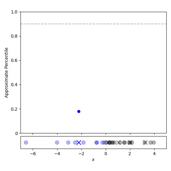
Figure 5: Estimating the 90th percentile is done by iterating through the t-digest centroids until the weight fraction has exceeded 90%. The approximate percentile is then estimated by linear interpolation.

The assumption being made in the above recurrence is that the centroid is not just the mean of the data in the cluster, but the median as well. Stated another way, if there are $n_{c_i}$ data points in the $i$th cluster, $n_{c_i}/2$ will be to the left of the centroid and $n_{c_i}/2$ will be to the right. Of course, this assumption need not hold and it is easy to find examples where it is false.

To get a sense of just how accurate these approximations are, we can visualise the corresponding cumulative distribution functions.

Imagine there are data from three different files stored on disk, each of which fit into memory but collectively are too large to load at once. Computing the t-digest of each set of data independently results in three different t-digests which can subsequently be merged into one. Note that this is different than simply concatenating all three data sources and computing a t-digest directly.

The leftmost panel of Figure 6 shows the histogram for three different random variables as well as the histogram for the collection of all of the variables together. This results in a distinctly bimodal distribution. The far right of this figure shows the approximation of the individual distributions by separate t-digests as well as the approximate distribution from merging these data structures. With only 30 data points, the t-digest approximation is able to estimate the empirical CDF very well.

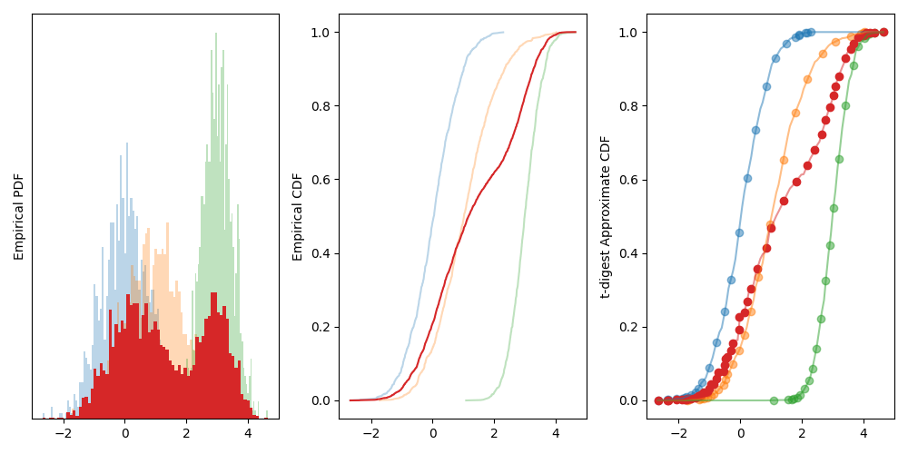
Figure 6: Left: Three histograms of different normal distributions along with the distribution of all three datasets together. Middle: The empirical CDFs of the distributions. Right: The approximate CDFs of the data computed using t-digests.

Conclusion

In summary, the t-digest is just a compressed representation of the data’s cumulative distribution function (CDF) that allows it to be easily combined with other t-digests. By choosing an appropriate scale parameter, the level of compression can be tuned to get the desired trade-off between memory usage and percentile accuracy.