Extending TensorFlow with Custom C++ Operations
- Software Engineering
DSE’s previous post blog post concluded by illustrating some of the limitations of the TensorFlow library. The off-the-shelf package is a great tool for deep learning, but with large model sizes these limitations become increasingly noticeable and require custom matrix operations to be implemented in the C++ source code.
Custom Op Motivations
Recall that only once all of the input tensors to a TensorFlow op are available can the op can be run and the output tensors computed. In particular, the op’s outputs are dependent only on its inputs and not influenced by any of the subsequent operations. One instance where this greedy strategy can lead to poor performance is computation involving many elementwise operations on the GPU (as in the case of the Gaussian Error Linear Unit mentioned in our previous post).
To further illustrate the need for custom operations, consider implementing a pairwise Manhattan distance function. The cdist function in the SciPy library is a generalisation of this, but, at the time of writing, there is no equivalent in TensorFlow.
This operation would be useful, for example, in a k-means implementation to find the distance between test data and the k centroids. It is also useful as a step during k-NN inference in order to compute the distances between each test data point and the training data.
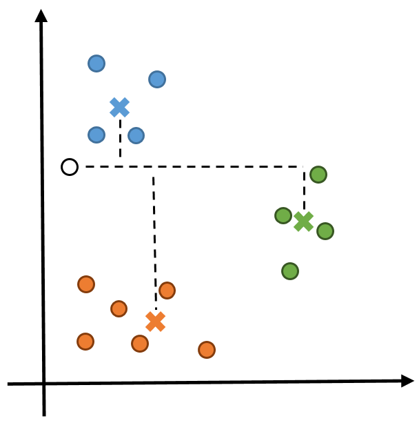
Figure 1: To compute the cluster membership of the new point (denoted by the black circle), the Manhattan distance to each centroid (denoted by crosses) must be computed. In this example, x has shape (3,2) and y has shape (1,2).
A first attempt at a pairwise distance operation in TensorFlow would be to use two for loops as in the tf_cdist function below. The body of the loop computes a single distance between vector i of the first collection and vector j of the second collection.
@tf.function
def tf_cdist(x, y):
    n, p = x.shape
    m, p = y.shape

    rows = []
    for i in range(n):
      row_elems = []
      for j in range(m):
        manhattan_dist_ij = tf.math.reduce_sum(tf.abs(x[i, :] - y[j, :]))
        row_elems.append(manhattan_dist_ij)
      rows.append(tf.stack(row_elems, axis=0))

    return tf.stack(rows, axis=0)
In practice, this solution is unacceptably slow for all but the smallest problem sizes as it leads to the creation of many small, but separate, operations in the compute graph as shown in Figure 2.
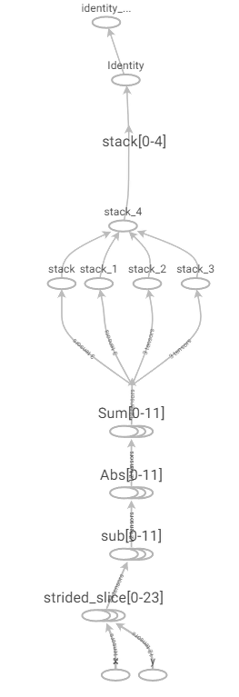
Figure 2: Naive Manhattan distance computation graph.
A more performant solution requires vectorising the operation. Instead of explicitly looping over each row of x and y, broadcasting can be used to create an intermediate 3d tensor with shape (n, m, p) containing each pair of absolute difference vectors. Each vector of absolute differences can then be summed to produce the final matrix of pairwise distances. This solution is outlined visually in Figure 3.
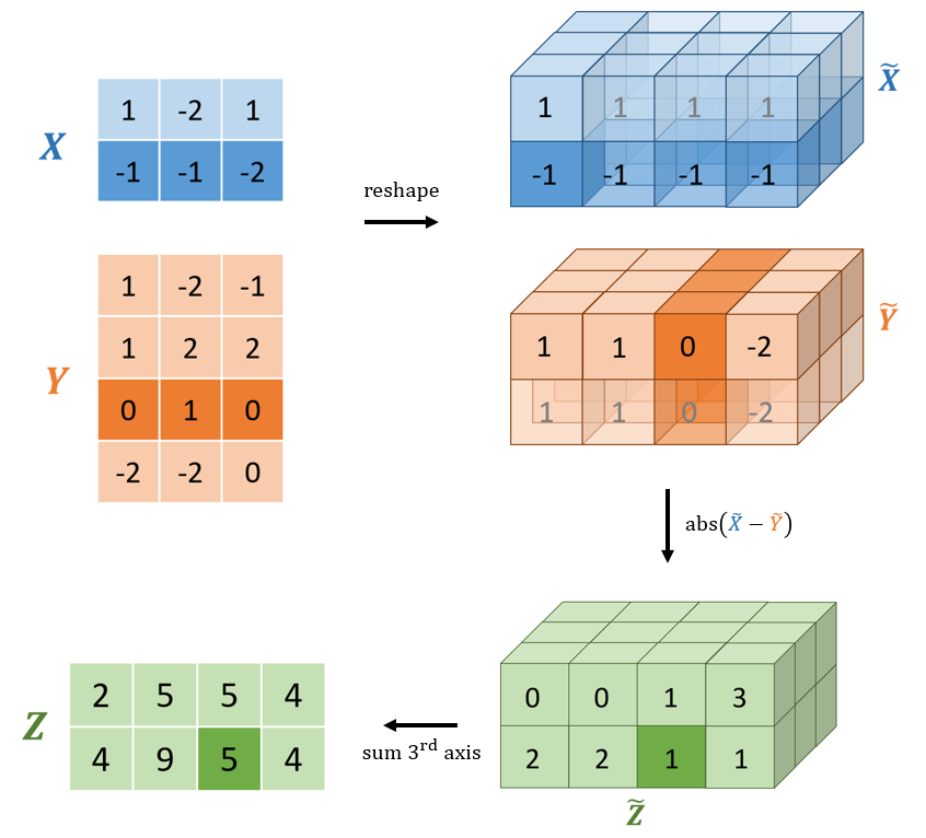
Figure 3: A visual diagram computing the Manhattan distance using broadcasting. The x and y matrices are reshaped to allow broadcasting. The two (conceptually) 3d tensors are subtracted and the absolute values computed. The resulting tensor requires storing all 24 elements (2 * 3 * 4). The last axis is then summed to produce the final pairwise Manhattan distance matrix. Note that the translucent cells are not actually created and thus require no extra memory. Conceptually, TensorFlow performs the subtraction as if these elements were present.
In TensorFlow, this can be implemented with the following code.
@tf.function
def tf_cdist_vectorised(x, y):
    n, p = tf.shape(x)
    m, p = tf.shape(y)
    z = tf.abs(tf.reshape(x, (n, 1, -1)) - tf.reshape(y, (1, m, -1)))

    return tf.sum(z, axis=-1)
This code results in a much simpler computation graph as shown in Figure 4.
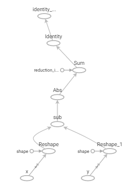
Figure 4: Vectorised Manhattan distance computation graph
Referring to Table 1, this implementation is significantly faster than the naive solution (for moderately sized inputs). The problem is that it requires O(mnp) space when the final output only requires O(mn). Since modern Nvidia GPUs have a memory limit of 32GB, large values of p severely limit the problem sizes on which the broadcast method can be used.
| n=m=32 | n=m=64 | n=m=128 | |
|---|---|---|---|
| Vectorised Batch Time (ms) | 1.1 | 2.0 | 5.8 |
| Loop Batch Time (ms) | 41.0 | 151.0 | 582.0 |
Table 1: Results from running the Manhattan distance implementations using TensorFlow 2.3 on a 32GB Tesla V100
The only way to avoid the extra factor of p memory usage in computing the pairwise distance function is to write a custom implementation of the operation that accumulates the p values directly into the (n,m) output tensor.
Anatomy of a TensorFlow Op
Each TensorFlow operation’s signature is defined in a C++ source file called <op_name>_ops.cc. The op registration defines
- input tensors
- output tensors
- allowable types of the tensors
- shape checking functionality (to ensure inputs and outputs conform to the shapes required by the computation)
Continuing with the pairwise Manhattan distance example, the op can be defined in TensorFlow with the following code:
// tensorflow/core/ops/pairwise_manhattan_distance_ops.cc
REGISTER_OP("PairwiseManhattanDistance")
    .Input("x: T")
    .Input("y: T")
    .Output("z: T")
    .Attr("T: {float, double}")
    .SetShapeFn([](InferenceContext* c) {
      ShapeHandle x, y;
      TF_RETURN_IF_ERROR(c->WithRank(c->input(0), 2, &x));
      TF_RETURN_IF_ERROR(c->WithRank(c->input(1), 2, &y));

      DimensionHandle n_x = c->Dim(x, 0);
      DimensionHandle n_y = c->Dim(y, 0);

      c->set_output(0, c->Matrix(n_x, n_y));

      return tensorflow::Status::OK();
    })
This defines an op that takes in two matrices (rank 2 tensors) that have matching second dimension. The operation produces a single output matrix whose first and second dimensions are the first dimension of the first and second input, respectively.
In addition to the op registration, each op has a corresponding op kernel (a separate concept from a CUDA kernel) which implements a method called Compute. This method defines how the op uses the inputs to produce the outputs. During execution of the graph, the TensorFlow session simply calls each op’s Compute method in succession.
Op Implementation
The implementation of a typical TensorFlow op follows a formulaic recipe. First, all of the op’s inputs are retrieved from a OpKernelContext object which is passed in to the Compute method.
// tensorflow/core/kernels/pairwise_manhattan_distance_ops.cc
namespace functor {
  void Compute(OpKernelContext* ctx) override {
      const Tensor* x_tensor = nullptr;
      const Tensor* y_tensor = nullptr;

      // Retrieve all of the inputs
      OP_REQUIRES_OK(ctx, ctx->input("x", &x_tensor));
      OP_REQUIRES_OK(ctx, ctx->input("y", &y_tensor));

      const int64 n = x_tensor->dim_size(0);
      const int64 m = y_tensor->dim_size(0);
      const int64 p = x_tensor->dim_size(1);

      ...
  }
}
The context object simply allows the op access to basic functionality such as querying the device, fetching the op’s inputs, and allocating space for new tensors. In this case, the OP_REQUIRES_OK macro ensures there are no failures when retrieving any of the inputs.
Next, space is allocated for the op’s outputs.
// tensorflow/core/kernels/pairwise_manhattan_distance_ops.cc
namespace functor {
  void Compute(OpKernelContext* ctx) override {
      ...

      // Allocate space for the output
      Tensor* z_tensor = nullptr;
      OP_REQUIRES_OK(
          ctx, ctx->allocate_output("z", TensorShape({n, m}),
                                    &z_tensor));

      ...
  }
}
The above code snippet allocates an output with the same number of rows as x and as many columns as y has rows. The OP_REQUIRES_OK macro ensures there are no allocation failures for any of the output tensors.
The last step is calling a device-specific implementation to fill the output tensors.
// tensorflow/core/kernels/pairwise_manhattan_distance_ops.cc
namespace functor {
  void Compute(OpKernelContext* ctx) override {
      ...

      const Device& device = ctx->eigen_device<Device>();

      // Call a device specific implementation to fill the output
      functor::ManhattanDistance<Device, T>(n, m, p)(
          ctx, device,
          x_tensor->matrix<T>(), y_tensor->matrix<T>(),
          z_tensor->matrix<T>());
  }
}
The actual computation logic is all handled by the call to the ManhattanDistance functor. This functor is templated on the device type, allowing the same op to have both a CPU and GPU implementation, but still have its Compute method invoked in a device independent way. This does mean that each op is usually implemented twice, once per device type. Because of the nature of CUDA programming, these implementations often look very different.
The following code shows a CPU implementation of the functor:
// tensorflow/core/kernels/pairwise_manhattan_distance.cc
template <typename T>
void ManhattanDistance(
    OpKernelContext* ctx, const CPUDevice& d,
    typename TTypes<T>::ConstMatrix x,
    typename TTypes<T>::ConstMatrix y,
    typename TTypes<T>::Matrix z) {

  auto n = x.dimension(0);
  auto m = y.dimension(0);
  auto p = y.dimension(1);

  T diff;
  T dist;
  for (int i = 0; i < n; i++) {
    for (int j = 0; j < m; j++) {
      dist = static_cast<T>(0);
      for (int k = 0; k < p; k++) {
        diff = x(i, k) - y(j, k);
        dist += Eigen::numext::abs(diff);
      }
      z(i, j) = dist;
    }
  }
}
The CPU version is almost the same as the first naive approach using TensorFlow. The key difference is that now the loops are being done in C++ inside a single op. In the TensorFlow implementation, the loops were executed in Python and created a new operation in the graph for each of the mn elements of the output. For large values of m and n, this is still too slow to be usable in practice.
The real performance benefits come when combining TensorFlow with hardware accelerators like GPUs. Nvidia GPUs consist of many streaming multiprocessors (SM) which can run computations completely in parallel. A GPU kernel executes on a single unit of computation called a thread. The GPU processor works on threads grouped into sets of 32, called warps. The multiprocessor schedules kernels to execute on collections of warps called a thread block. The set of all the blocks making up the computation is called a grid.
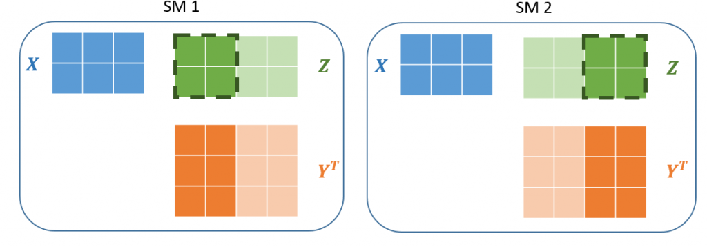
Figure 5: Left A block of 4 threads are run concurrently on the first of the GPU’s SMs. Each of the threads compute a single value of the output. Right Another block of 4 threads computes the remaining outputs on the second SM. Since the blocks are 2×2, each block only needs to load a subet of the Y matrix values. Together the blocks completely tile the output matrix forming a grid
The following code is a basic implementation of a CUDA kernel to compute the pairwise Manhattan distance.
template <typename T>
__global__ void manhattan_distance(
    const T* x,
    const T* y,
    T* z,
    const int n,
    const int m,
    const int p) {

  const int i = blockIdx.y * blockDim.y + threadIdx.y;
  const int j = blockIdx.x * blockDim.x + threadIdx.x;
  const int index = i * m + j;

  if ((i >= n) || (j >= m)) return;

  T dist = 0.0;
  T diff;
  for (int k = 0; k < p; k++) {
    diff = x[i * p + k] - y[j * p + k];  // x[i, k] - y[j, k]
    dist += Eigen::numext::abs(diff);
  }

  z[index] = dist;
}
Rather than Eigen tensors, the kernel takes in a flattened buffer of values laid out in row-major order (see the previous post for details). The first three lines of the kernel use the location of the thread’s block in the grid as well as the block shapes to work out which element of the output the particular thread should compute. The remaining code is equivalent to the inner loop of the CPU version. The reason that there is no loop over the rows of x and y as in the CPU code is that CUDA handles this implicitly when the kernel is declared with its grid and block dimensions.
Finally, this CUDA kernel would be called by a ManhattanDistance functor as in the following code example.
// tensorflow/core/kernels/pairwise_manhattan_distance_gpu.cu.cc
template <typename T>
void ManhattanDistance(
    OpKernelContext* ctx, const GPUDevice& d,
    typename TTypes<T>::ConstMatrix x,
    typename TTypes<T>::ConstMatrix y,
    typename TTypes<T>::Matrix z) {
  const auto& cu_stream = GetGpuStream(ctx);

  const int n = x.dimension(0);
  const int m = y.dimension(0);
  const int p = x.dimension(1);

  dim3 block_dim_2d(32, 8);

  auto grid_dim_x = (m + block_dim_2d.x - 1) / block_dim_2d.x;
  auto grid_dim_y = (n + block_dim_2d.y - 1) / block_dim_2d.y;
  dim3 grid_dim_2d(grid_dim_x, grid_dim_y);

  manhattan_distance<T><<<grid_dim_2d, block_dim_2d, 0, cu_stream>>>(
      x.data(), y.data(), z.data(), n, m, p);
}
The Backward Step
In deep learning, having just the op’s implementation is insufficient for model training. In addition, we need a way to differentiate through the operation to compute the gradients with respect to all of the various model parameters. The PairwiseManhattanDistance definition makes no mention of the gradient or a backward method. With a few exceptions, for every op registration there is a corresponding gradient operation. Exceptions include operations that define their gradients in Python, operations that have no gradient at all (e.g. argsort), and operations that are only run in inference (the PairwiseManhattanDistance could be an instance of this).
The definition of the gradient op for the PairwiseManhattanDistance looks very similar to the forward op’s registration.
REGISTER_OP("PairwiseManhattanDistanceGrad")
    .Input("x: T")
    .Input("y: T")
    .Input("z_grad: T")
    .Output("x_grad: T")
    .Output("y_grad: T")
    .Attr("a: int = 1")
    .Attr("T: {float, double}")
    .SetShapeFn([](InferenceContext* c) {
      ShapeHandle x, y;
      TF_RETURN_IF_ERROR(c->WithRank(c->input(0), 2, &x));
      TF_RETURN_IF_ERROR(c->WithRank(c->input(1), 2, &y));

      DimensionHandle n_x = c->Dim(x, 0);
      DimensionHandle n_y = c->Dim(y, 0);
      DimensionHandle feature_dim = c->Dim(x, 1);

      c->set_output(0, c->Matrix(n_x, feature_dim));
      c->set_output(1, c->Matrix(n_y, feature_dim));

      return tensorflow::Status::OK();
    })
One thing to note is the duality between this operation and its forward version. The PairwiseManhattanDistanceGrad takes as input, the gradient with respect to the original op’s output. The outputs are the gradients with respect to the original op’s input.
As an aside on the variable naming convention, it might be more explicit to write z_grad as dLdz in order to emphasise that it is a gradient of the loss with respect to z. However, in TensorFlow it is understood that all gradients are of the loss function with respect to some variable, so the reference to the loss is always omitted in the names of the gradient variable.
When it comes to the implementation of the gradient, it does not matter whether it comes from a table of matrix derivatives, is derived from the delta-epsilon definition, or found on an old StackOverflow post. The important point is that it must come from somewhere. TensorFlow’s automatic differentiation simply orchestrates the calling of gradient operations, but it does not have any intrinsic understanding of any of the ops’ logic. This means that the op gradient is only as good as the hand coded implementation. If the implementation is slow, has suboptimal space usage, or is just plain incorrect, the automatic differentiation framework will not be of any use.
Conclusion
While TensorFlow is a valuable tool for deep learning, in practice, its limitations become apparent as the models become increasingly large and exotic. The main inefficiencies come from the ops being greedily executed in sequence with little context of the operations upstream or downstream. But many of the difficulties can be overcome with additional effort. While the work to create an operation is significant, involving detailed knowledge of CUDA programming, the benefits can be immense, as it enables more efficient use of the hardware than is possible with the standard TensorFlow distribution. In the future, more sophisticated graph optimisation and compilation may be able to remove these inefficiencies and reduce the number of situations where a custom op implementation is necessary.