Implementing SLIDE
- Software Engineering
The increasing size and training time of neural network models has lead to increasing reliance on specialised hardware.
GPUs are one of many high throughput devices designed to perform massively parallel operations such as large matrix multiplications which form the backbone of machine learning. Despite the high cost, GPU training is significantly faster than CPU and is often the only viable option for model training. The sublinear deep learning engine (SLIDE) is an algorithm designed to efficiently train neural networks entirely on CPU.
The authors of the SLIDE algorithm claim to achieve faster convergence with their C++ implementation of SLIDE compared to an equivalent TensorFlow model trained on the GPU. Specifically, the authors demonstrate a speedup on tasks which have an enormous number of possible classes, referred to as extreme classification tasks.
We attempted to implement SLIDE in Julia – a relatively niche and easy-to-use programming language which claims to achieve speeds competitive with C++. The goal of the project was to check if SLIDE does perform as well as the authors claim as well as to directly benchmark Julia against C++.
Idea behind SLIDE
Neural network training is divided into two parts; the forward pass to compute the outputs and the backward pass to compute the weight updates. In the forward pass, the $i$th output of layer $ell$ is computed by equation 1
where $z$ is an input vector to the layer, $g$ is the non-linear activation function of the layer, and $w_i$ and $b_i$ are the weights and biases of the $i$th output respectively.
The intuition behind SLIDE is that different neurons are responsible for detecting different features and only those having relevant features for a given input will have high activations. The remaining neurons will have much smaller activations and as a result, will propagate weaker signal to the subsequent layers. In fact, in large neural networks there might be a significant proportion of inactive neurons which means that most of the computations will be superfluous and won’t contribute to the final prediction.
What if we could choose a subset of neurons that are most likely to be active before performing all of the computations? This way, we would avoid having to take inner products of an input with all of the weights, but instead do it only for selected neurons. The SLIDE algorithm attempts to predict which neurons maximise the inner product with an input by using locality sensitive hashing(LSH). A locality sensitive hash ensures that “similar” vectors have the same hash code while dissimilar objects have different hash codes.
If we use an inner product as the similarity measure, the problem comes down to selecting the weight vectors which have the same hash as an intermediate activation in the given layer.
SLIDE details
LSH
Ideally, we would like our randomised hash function $h$ to satisfy following property for any input $z$ and neuron weight vector $w$:
where $f$ is a monotonically increasing function and sim is the predefined similarity measure. The term $P(h(z) = h(w))$ is referred to as the collision probability. The assumption about function $f$ guarantees that the more similar two vectors are, the higher the probability that they will have the same hash code.
Because the hashing is probabilistic, it is always possible that two similar (but non-identitical) vectors end up with different hash codes. To reduce this possibility, we can hash the vector multiple times. Specifically, the LSH algorithm can be parameterised by a pair $(K, L)$ which corresponds to the creation of $Ktimes L$ independent hash functions.
A single hash is created by concatenating outputs of $K$ different hash functions and then constructing $L$ hashes of length $K$, each corresponding to its own hash table. When given an input vector, we can take the union of neurons from selected buckets of all $L$ tables. The larger $K$ is, the lower the probability that a dissimilar vector accidentally matches the hash code, reducing the number of false positives. In contrast, choosing a larger value of $L$ increases the number of retrieved elements, improving recall.
In SLIDE, at the beginning of training we compute hashes in each hashing layer for all weight vectors and store them in $L$ hash tables as illustrated in Figure 1. As the training proceeds and weights are updated during back propagation, the weight vectors’ hash codes may change so this hashing step must be repeated periodically.
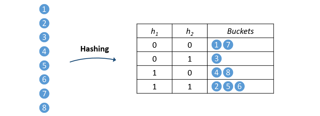
Figure 1: Preprocessing phase when all neurons are hashed and stored in the hashtables.
SimHash
It is difficult to come up with an efficient hashing function satisfying the LSH property for maximum inner product search (MIPS), so in practice other similarity measures are used. An example of such a measure is the cosine similarity which is shown in Figure 2.
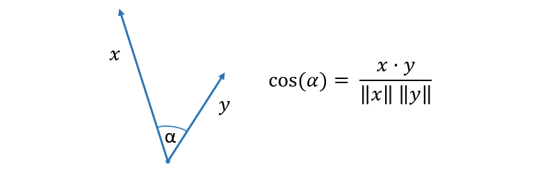
Figure 2: Cosine similarity is defined as the cosine of the angle between two vectors.
In general, maximising cosine similarity is not equivalent to maximising the inner product unless all of the neuron weight vectors have equal $L_2$ norm. In practice however, it can serve as a good approximation.
SimHash is a relatively simple and fast algorithm with the LSH property that approximately solves the problem of finding vectors with the highest cosine similarity to a given vector. During initialisation, we sample a random hyperplane and assign $0$ or $1$ based on which side of the hyperplane a given vector lies.
This information can be computed by taking the sign of the inner product of the vector with the hyperplane’s normal vector. To accelerate this computation, it is common to sample hyperplanes with a normal vector having components that are $+1$, $0$ or $-1$.
From Figure 3, we see that vectors with a small angle between them have a very low chance of lying on opposite sides of a random hyperplane. Conversely, vectors with a large angle between them are very likely to be on opposite sides of a randomly selected hyperplane.
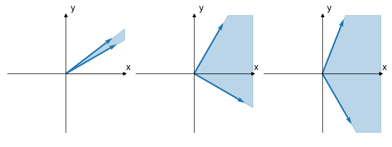
Figure 3: The light blue region depicts the space in which a hyperplane needs to lie in order to separate the two vectors. As the angle between the two vectors increases (from left to right), the space in which a hyperplane can divide the vectors into two subsets grows larger.
Using a single hyperplane will yield just a single bit hash code. This has the obvious disadvantage that, by chance, two dissimilar vectors could end up on the same side of the hyperplane and thus hash to the same value. Choosing $K$ random hyperplanes will produce a $K$-bit hash as illustrated in Figure 4, reducing the likelihood of these false positives.
Figure 4: Each hyperplane divides the vectors into two subsets. Using 5 different hyperplanes produces a 5 bit hash for each vector. Each row of the table corresponds to the hash of a vector. The vectors are ordered by their angle measured anti-clockwise from the positive x-axis.
Training neural networks with LSH
SLIDE works by replacing the usual matrix-vector multiplications in a feed forward neural network with LSH operations. However, performance benefits are only seen when the layer has sufficiently large output dimension such that sampling achieves significant sparsity.
In SLIDE, the authors only use hashing in the final layer of their network because of the enormous number of classes in the extreme classification datasets they benchmark against.
As described previously, in the pre-processing phase all weights within a layer are hashed and stored in the hashtables. In the forward pass the only thing we have to do is feed our hashing function with a vector of features obtained from the previous layer. This is illustrated in Figure 5.
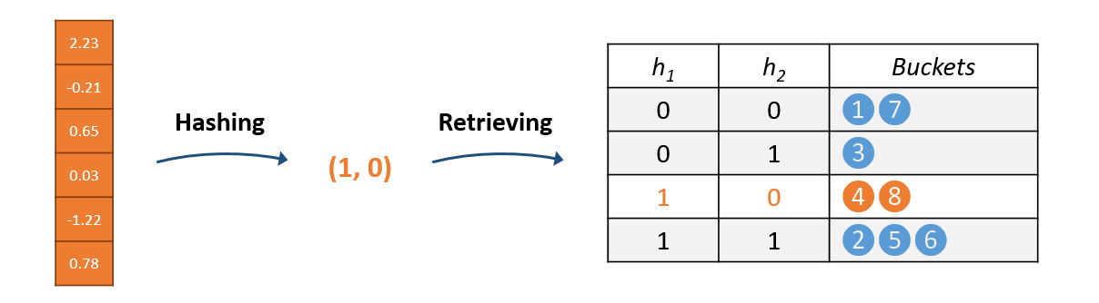
Figure 5: Neurons having the same hash as the input to the layer are retrieved.
Rather than computing the full matrix-vector multiplication, we retrieve only the neurons (i.e. rows of the weight matrix) with at least one hash code matching the input and compute the inner products. All other neurons are considered inactive and have their activations treated as $0$.
This can significantly reduce the number of floating point operations. Similarly, backpropagation and weight updates are performed only for active neurons.
For each instance of the batch, a different set of neurons is sampled. Assuming the number of neurons is large, there is a only a small probability that the sets of neurons activated by each instance have any overlap.
This observation allows us to asynchronously update the gradients in parallel for each instance since the sparsity of the updates makes it unlikely to impact training convergence. As shown in Figure 6, each training instance can be processed by a single thread to increase throughput.
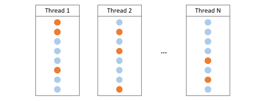
Figure 6: Each thread samples different subsets of neurons within a layer.
Results
Following the authors, we benchmark models on two extreme classification datasets: Delicious-200K and Amazon-670K.
In our experiments we use similar hyperparameters to the ones used in the paper. In Figure 7, we plot test accuracy on Delicious-200K achieved by the authors’ C++ implementation, our Julia implementaiton, and a vanilla neural network trained on a V100 GPU using Julia’s ML framework, Flux. Accuracy is measured only for the most probable class predicted by a model.
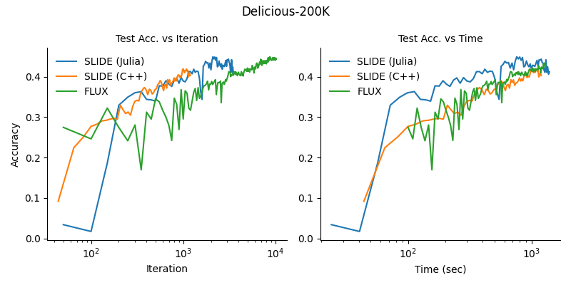
Figure 7: The Julia implementation of SLIDE converges similarly (albeit slightly faster) on the Delicious-200K dataset.
The above figure shows that SLIDE can converge faster than a regular feed-forward neural network trained on a GPU with this dataset. However, we found that the dataset suffers from severe class imbalance. In fact, one class appears in almost 40% of test instances suggesting that even simple models could be competitive. We also benchmarked our implementation against the Amazon-670k dataset, which has a more even class distribution, but did not manage to reproduce the accuracy of the original C++ implementation. These results are shown in Figure 8.
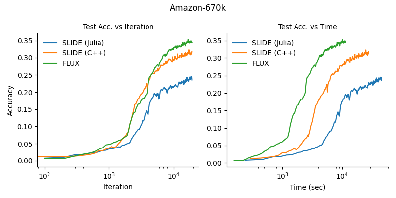
Figure 8: Convergence of the Julia SLIDE implementation was markedly worse than the authors’ implementation on the more difficult Amazon-670K dataset. The Flux GPU implementation of the full dense model shows the best wall time convergence.
We also considered using various other hash functions or hyperparameters but none of these experiments matched the training curves of the original implementation. We spotted a number of implementation details in the authors’ code which might suggest that training a network with an LSH module is in fact a very difficult task. Even though SLIDE proved to work well on one particular data task, the results indicate it has difficulty efficiently solving more challenging extreme classification tasks.
Performance
One of the most challenging parts of the SLIDE implementation was getting performant Julia code that could compete with the original C++ implementation. In order to do this, we performed a number of additional optimisations on top of those originally used.
Rather than treat the weights as collections of neurons we instead stored them as a dense matrix in order to leverage vectorised linear algebra operations. We also made heavy use of sparsity by storing each state in a compact format which saves computation and reduces memory usage.
Generally, we found careful memory management to be crucial to writing fast Julia code. In Julia, once garbage collection begins, all threads are paused, severely impacting the performance. To avoid this, we needed to pre-allocate working arrays whenever possible. We managed to obtain up to 30x speed-up compared to our initial implementation of SLIDE.
In Table 1 we compare two implementations by measuring average time per iteration. This metric also includes an amortised cost of hashtable updates and reconstructions which occur once every 50 iterations in both models. We managed to match, and in some cases, exceed the performance of C++ with our Julia implementation.
| Model | Delicious | Amazon | |
|---|---|---|---|
| C++, 8-threads | 0.9s | 1.72s | |
| Julia, 8-threads | 0.72s | 1.63s |
| Model | Delicious | Amazon | |
|---|---|---|---|
| C++, 40-threads | 0.43s | 0.57s | |
| Julia, 40-threads | 0.57s | 1.4s |
Table 1: Average time per iteration on different CPUs.
Conclusion
By leveraging sparsity using intelligent sampling, SLIDE aims speed up neural network components and enable the use of CPUs to train neural networks.
While SLIDE’s usage is constrained to a handful of domain-specific extreme classification tasks, it is undoubtedly a noteworthy attempt to break GPU supremacy.